
When working with numbers in Microsoft Excel, you can highlight negative numbers in red; this makes it easier to read data. There are a few techniques that you can use to highlight negative numbers, such as using conditional formatting, inbuilt number formatting, and using custom formatting. The Conditional Formatting feature easily spots trends and patterns in your data usage bars, colors, and icons to visually highlight important values. It is applied to cells based on the values it holds.
How to highlight Negative numbers in Excel
You can highlight cells with negative values in Excel and make them stand out in Red using one of these methods:
- Using Conditional Formatting
- Using Custom Formatting
1] Using Conditional Formatting
In Excel, you can format a negative number by creating a Conditional Formatting rule.
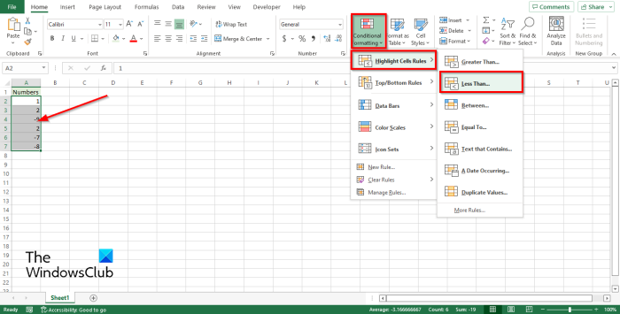
- Select the range of cells containing the numbers.
- On the Home tab, in the Styles group, click the Conditional Formatting button.
- Hover your cursor over Highlight cell rules and then click Less Then.
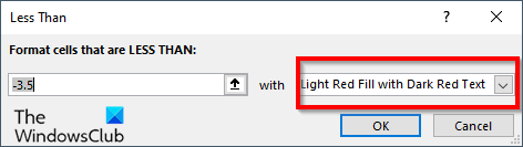
- A Less Than dialog box will open, click the drop-down arrow, and select a highlight, for instance, Light red fill with dark red text.
- Click OK.
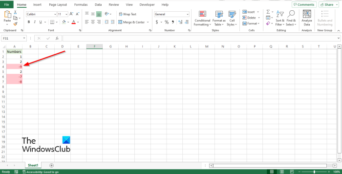
All the cells of negative numbers will become red, while the positive numbers will remain the same.
2] Using custom formatting
You can create your own custom format in Excel to highlight negative numbers.
Select the range of cells containing the numbers.
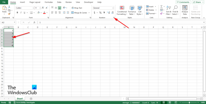
On the Home tab in the Numbers group, click the small arrow button or press the shortcut keys Ctrl + 1.
A Format Cells dialog box will open.
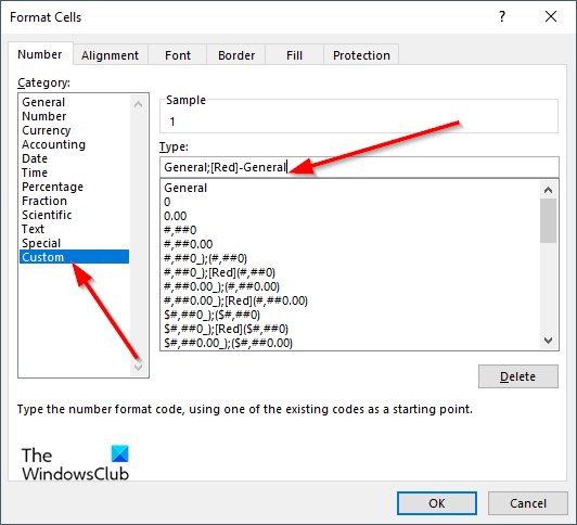
On the Number tab, select Custom on the left pane.
On the right in the Type section, type into the entry box the format code General;[Red]-General.
Then click OK.
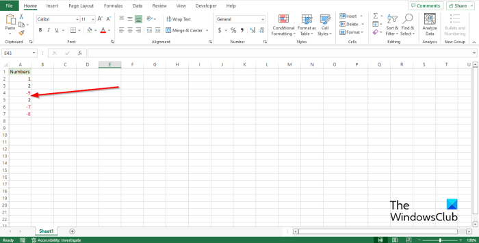
All the negative numbers will become red, while the positive numbers will remain the same.
We hope this tutorial helps you understand how to highlight negative numbers in Excel; if you have questions about the tutorial, let us know in the comments.
How do I make negative numbers red in Excel?
You can highlight cells with negative values in Excel and make them stand out in Red using one of these methods:
- Using Conditional Formatting
- Using Custom Formatting
How do I apply conditional color in Excel?
If you want to add condition color in Excel, follow the steps below:
- Click Conditional Formatting button in the Styles group.
- Click New Rule in the menu.
- Select a style, for example, 3-Color Scale, select the conditions that you want, and then click OK.
What is highlight cell rules in Excel?
When you click the Conditional Formatting button in Excel, you will see the Highlight Cell Rules feature. The Highlight Cell Rule feature is a type of conditional formatting used to change the appearance of cells in a range based on your specified conditions.
What are the four types of conditional formatting?
There are five types of conditional formatting visualization available; these are Background Shading of cells, Foreground shading of cells, Data bars, and Icons, which have four image types and values.
READ: Change Cell Background Color in Excel with VBA Editor
How do I automatically highlight cells in Excel based on value?
Follow the steps below to automatically highlight cells in Excel based on value.
- On the Home tab in the Styles group, click the Conditional Formatting button.
- Click Manage Rules.
- Create a new rule.
- In the Select a rule display box, select use formula to determine which cells to format.
- Enter a value for instance =A2=3.
- Click the Format button.
- Click the Fill tab and then choose a color.
- Click Ok for both boxes.
- The color of the cell will change.